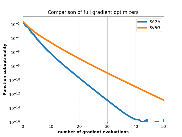
SAGA vs SVRG

A comparison between two variance-reduced stochastic gradient methods: SAGA (implemented in copt.minimize_saga()) and SVRG (implemented in copt.minimize_svrg()). The problem solved in this case is the sum of a logistic regression and an L1 norm (sometimes referred to as sparse logistic)

import copt as cp
import matplotlib.pyplot as plt
import numpy as np

# .. construct (random) dataset ..
import copt.loss
import copt.penalty

n_samples, n_features = 1000, 200
np.random.seed(0)
X = np.random.randn(n_samples, n_features)
y = np.random.rand(n_samples)

# .. objective function and regularizer ..
f = copt.loss.LogLoss(X, y)
g = copt.penalty.L1Norm(1.0 / n_samples)

# .. callbacks to track progress ..
cb_saga = cp.utils.Trace(lambda x: f(x) + g(x))
cb_svrg = cp.utils.Trace(lambda x: f(x) + g(x))

# .. run the SAGA and SVRG algorithms ..
step_size = 1.0 / (3 * f.max_lipschitz)
result_saga = cp.minimize_saga(
    f.partial_deriv,
    X,
    y,
    np.zeros(n_features),
    prox=g.prox_factory(n_features),
    step_size=step_size,
    callback=cb_saga,
    tol=0,
    max_iter=100,
)

result_svrg = cp.minimize_svrg(
    f.partial_deriv,
    X,
    y,
    np.zeros(n_features),
    prox=g.prox_factory(n_features),
    step_size=step_size,
    callback=cb_svrg,
    tol=0,
    max_iter=100,
)


# .. plot the result ..
fmin = min(np.min(cb_saga.trace_fx), np.min(cb_svrg.trace_fx))
plt.title("Comparison of full gradient optimizers")
plt.plot(cb_saga.trace_fx - fmin, lw=4, label="SAGA")
# .. for SVRG we multiply the number of iterations by two to ..
# .. account for computation of the snapshot gradient ..
plt.plot(
    2 * np.arange(len(cb_svrg.trace_fx)), cb_svrg.trace_fx - fmin, lw=4, label="SVRG"
)
plt.ylabel("Function suboptimality", fontweight="bold")
plt.xlabel("number of gradient evaluations", fontweight="bold")
plt.yscale("log")
plt.ylim(ymin=1e-16)
plt.xlim((0, 50))
plt.legend()
plt.grid()
plt.show()

Estimated memory usage: 82 MB