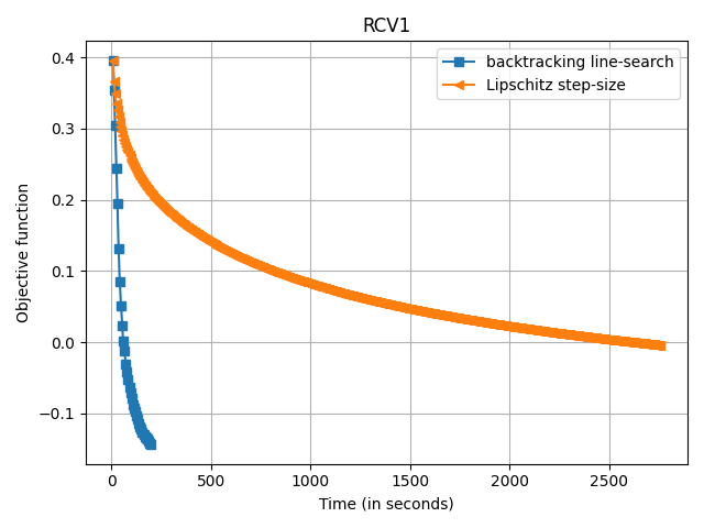
Benchmark of Pairwise Frank-Wolfe variants for sparse logistic regression

Speed of convergence of different Frank-Wolfe variants on various problems with a logistic regression loss (copt.utils.LogLoss()) and a L1 ball constraint (copt.utils.L1Ball()).

• 
• 
• 
• 

Out:

Running on the RCV1 dataset
(697641, 47236)
Sparsity of solution: 0.0023499026166483193
0.30717282923725736
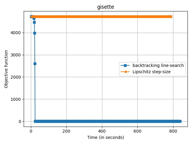
Running on the gisette dataset
(7000, 5000)
/workspace/copt/frank_wolfe.py:71: RuntimeWarning: divide by zero encountered in double_scalars
  tmp = (certificate ** 2) / (2 * (old_f_t - f_t) * norm_update_direction)
Sparsity of solution: 0.0002
4734.010016774253
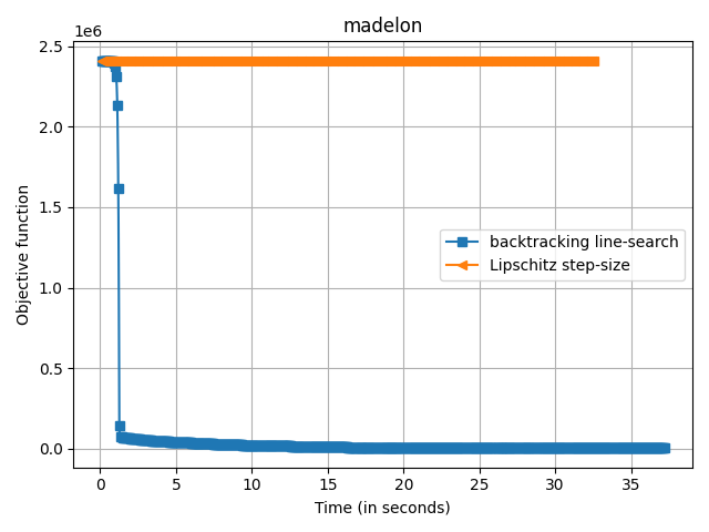
Running on the madelon dataset
(2600, 500)
Sparsity of solution: 0.004
2408517.4809582275
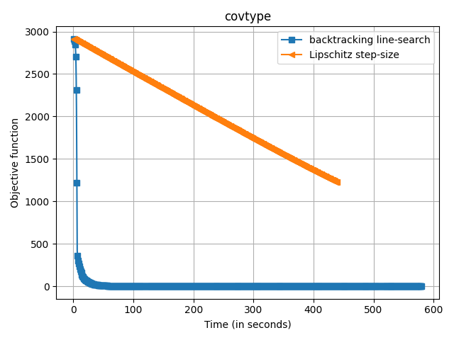
Running on the covtype dataset
(581012, 54)
Sparsity of solution: 0.037037037037037035
1225.9508846942538

import matplotlib.pyplot as plt
import numpy as np
import copt as cp

# .. datasets and their loading functions ..
# .. last value si the regularization parameter ..
# .. which has been chosen to give 10% feature sparsity ..
import copt.constraint
import copt.loss

datasets = (
    {
        "name": "RCV1",
        "loader": cp.datasets.load_rcv1,
        "alpha": 1e3,
        "max_iter": 5000,
        "f_star": 0.3114744279728717,
    },
    {
        "name": "gisette",
        "loader": cp.datasets.load_gisette,
        "alpha": 1e4,
        "max_iter": 5000,
        "f_star": 2.293654421822428,
    },
    {
        "name": "madelon",
        "loader": cp.datasets.load_madelon,
        "alpha": 1e4,
        "max_iter": 5000,
        "f_star": 0.0,
    },
    {
        "name": "covtype",
        "loader": cp.datasets.load_covtype,
        "alpha": 1e4,
        "max_iter": 5000,
        "f_star": 0,
    },
)


variants_fw = [
    ["backtracking", "backtracking line-search", "s"],
    ["DR", "Lipschitz step-size", "<"],
]

for d in datasets:
    plt.figure()
    print("Running on the %s dataset" % d["name"])

    X, y = d["loader"]()
    print(X.shape)
    n_samples, n_features = X.shape

    l1_ball = copt.constraint.L1Ball(d["alpha"])
    f = copt.loss.LogLoss(X, y)
    x0 = np.zeros(n_features)
    x0[0] = d["alpha"]  # start from a (random) vertex

    for step, label, marker in variants_fw:

        cb = cp.utils.Trace(f)
        sol = cp.minimize_frank_wolfe(
            f.f_grad,
            x0,
            l1_ball.lmo_pairwise,
            callback=cb,
            step=step,
            lipschitz=f.lipschitz,
            max_iter=d["max_iter"],
            verbose=True,
            tol=0,
        )

        plt.plot(
            cb.trace_time,
            np.array(cb.trace_fx) - d["f_star"],
            label=label,
            marker=marker,
            markevery=10,
        )

    print("Sparsity of solution: %s" % np.mean(np.abs(sol.x) > 1e-8))
    print(f(sol.x))
    plt.legend()
    plt.xlabel("Time (in seconds)")
    plt.ylabel("Objective function")
    plt.title(d["name"])
    plt.tight_layout()  # otherwise the right y-label is slightly clipped
    #    plt.xlim((0, 0.7 * cb.trace_time[-1]))  # for aesthetics
    plt.grid()
    plt.show()

Estimated memory usage: 1519 MB