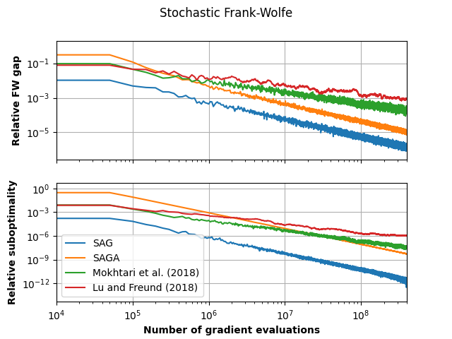
Comparison of variants of Stochastic FW

The problem solved in this case is a L1 constrained logistic regression (sometimes referred to as sparse logistic regression).

Out:

Running SAGFW
Running SAGAFW
Running MHK
Running LF

import copt as cp
import matplotlib.pyplot as plt
import numpy as np
import sklearn


# .. construct (random) dataset ..
import copt.constraint
import copt.loss

n_samples, n_features = 500, 200
np.random.seed(0)
X = np.random.randn(n_samples, n_features)
y = np.random.rand(n_samples)
batch_size = n_samples // 10
n_batches = n_samples // batch_size
max_iter = int(1e6)
freq = max(n_batches, max_iter // 1000)

# .. objective function and regularizer ..
f = copt.loss.LogLoss(X, y)
constraint = copt.constraint.L1Ball(1.)


# .. callbacks to track progress ..
def fw_gap(x):
    _, grad = f.f_grad(x)
    return constraint.lmo(-grad, x)[0].dot(-grad)


class TraceGaps(cp.utils.Trace):
    def __init__(self, f=None, freq=1):
        super(TraceGaps, self).__init__(f, freq)
        self.trace_gaps = []

    def __call__(self, dl):
        if self._counter % self.freq == 0:
            self.trace_gaps.append(fw_gap(dl['x']))
        super(TraceGaps, self).__call__(dl)


cb_sfw_SAG = TraceGaps(f, freq=freq)
cb_sfw_SAGA = TraceGaps(f, freq=freq)
cb_sfw_mokhtari = TraceGaps(f, freq=freq)
cb_sfw_lu_freund = TraceGaps(f, freq=freq)

# .. run the SFW algorithm ..
print("Running SAGFW")
result_sfw_SAG = cp.minimize_sfw(
    f.partial_deriv,
    X,
    y,
    np.zeros(n_features),
    constraint.lmo,
    batch_size,
    callback=cb_sfw_SAG,
    tol=0,
    max_iter=max_iter,
    variant='SAG'
)

print("Running SAGAFW")
result_sfw_SAGA = cp.minimize_sfw(
    f.partial_deriv,
    X,
    y,
    np.zeros(n_features),
    constraint.lmo,
    batch_size,
    callback=cb_sfw_SAGA,
    tol=0,
    max_iter=max_iter,
    variant='SAGA'
)

print("Running MHK")
result_sfw_mokhtari = cp.minimize_sfw(
    f.partial_deriv,
    X,
    y,
    np.zeros(n_features),
    constraint.lmo,
    batch_size,
    callback=cb_sfw_mokhtari,
    tol=0,
    max_iter=max_iter,
    variant='MHK'
)

print("Running LF")
result_sfw_lu_freund = cp.minimize_sfw(
    f.partial_deriv,
    X,
    y,
    np.zeros(n_features),
    constraint.lmo,
    batch_size,
    callback=cb_sfw_lu_freund,
    tol=0,
    max_iter=max_iter,
    variant='LF'
)
# .. plot the result ..
max_gap = max(cb_sfw_SAG.trace_gaps[0],
              cb_sfw_mokhtari.trace_gaps[0],
              cb_sfw_lu_freund.trace_gaps[0],
              cb_sfw_SAGA.trace_gaps[0])

max_val = max(cb_sfw_SAG.trace_fx[0],
              cb_sfw_mokhtari.trace_fx[0],
              cb_sfw_lu_freund.trace_fx[0],
              cb_sfw_SAGA.trace_fx[0])

min_val = min(np.min(cb_sfw_SAG.trace_fx),
              np.min(cb_sfw_mokhtari.trace_fx),
              np.min(cb_sfw_lu_freund.trace_fx),
              np.min(cb_sfw_SAGA.trace_fx),
              )

fig, (ax1, ax2) = plt.subplots(2, sharex=True)
fig.suptitle('Stochastic Frank-Wolfe')

ax1.plot(freq * batch_size * np.arange(len(cb_sfw_SAG.trace_gaps)), np.array(cb_sfw_SAG.trace_gaps) / max_gap, label="SAG")
ax1.plot(freq * batch_size * np.arange(len(cb_sfw_SAGA.trace_gaps)), np.array(cb_sfw_SAGA.trace_gaps) / max_gap, label="SAGA")
ax1.plot(freq * batch_size * np.arange(len(cb_sfw_mokhtari.trace_gaps)), np.array(cb_sfw_mokhtari.trace_gaps) / max_gap, label='Mokhtari et al. (2018)')
ax1.plot(freq * batch_size * np.arange(len(cb_sfw_lu_freund.trace_gaps)), np.array(cb_sfw_lu_freund.trace_gaps) / max_gap, label='Lu and Freund (2018)')
ax1.set_ylabel("Relative FW gap", fontweight="bold")
ax1.set_yscale('log')
ax1.set_xscale('log')
ax1.grid(True)

ax2.plot(freq * batch_size * np.arange(len(cb_sfw_SAG.trace_fx)), (np.array(cb_sfw_SAG.trace_fx) - min_val) / (max_val - min_val), label="SAG")
ax2.plot(freq * batch_size * np.arange(len(cb_sfw_SAGA.trace_fx)), (np.array(cb_sfw_SAGA.trace_fx) - min_val) / (max_val - min_val), label="SAGA")
ax2.plot(freq * batch_size * np.arange(len(cb_sfw_mokhtari.trace_fx)), (np.array(cb_sfw_mokhtari.trace_fx) - min_val) / (max_val - min_val), label='Mokhtari et al. (2018)')
ax2.plot(freq * batch_size * np.arange(len(cb_sfw_lu_freund.trace_fx)), (np.array(cb_sfw_lu_freund.trace_fx) - min_val) / (max_val - min_val), label='Lu and Freund (2018)')
ax2.set_ylabel("Relative suboptimality", fontweight="bold")
ax2.set_xlabel("Number of gradient evaluations", fontweight="bold")
ax2.set_yscale('log')
ax2.set_xscale("log")
ax2.grid(True)

plt.xlim(1e4, 4e8)
plt.legend()
plt.show()

Estimated memory usage: 9 MB