Combining COPT with JAX

This example shows how JAX can be used within COPT to compute the gradients of the objective function.

Out:

WARNING:absl:No GPU/TPU found, falling back to CPU. (Set TF_CPP_MIN_LOG_LEVEL=0 and rerun for more info.)

import jax
from jax import numpy as np
import numpy as onp
import matplotlib.pyplot as plt
from sklearn import datasets
import copt as cp

# .. construct (random) dataset ..
import copt.penalty

X, y = datasets.make_regression()
n_samples, n_features = X.shape


def loss(w):
    """Squared error loss."""
    z = np.dot(X, w) - y
    return np.sum(z * z) / n_samples


# .. use JAX to compute the gradient of loss value_and_grad ..
# .. returns both the gradient and the objective, which is ..
# .. the format that COPT accepts ..
f_grad = jax.value_and_grad(loss)

w0 = onp.zeros(n_features)

l1_ball = copt.penalty.L1Norm(0.1)
cb = cp.utils.Trace(lambda x: loss(x) + l1_ball(x))
sol = cp.minimize_proximal_gradient(
    f_grad, w0, prox=l1_ball.prox, callback=cb, jac=True
)
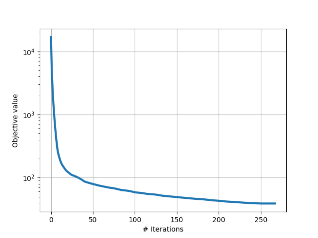
plt.plot(cb.trace_fx, lw=3)
plt.yscale("log")
plt.xlabel("# Iterations")
plt.ylabel("Objective value")
plt.grid()
plt.show()

Estimated memory usage: 78 MB